\[\definecolor{dodgerblue}{30,144,255} \definecolor{hotpink}{255,105,180}\]

Euler's Method

In most cases, we will be presented with a differential equation that cannot be solved in finite terms, that is, as a finite combination of elementary functions. Even when we can find such a solution, it may then be the case that we cannot visualize the solution without the aid of a computer, so the solution itself is really not useful by itself. As we can see, we can get a graph of any first order differential equation to any level of precision we may want, without having to do any differentiation or antidifferentiation.

As we saw in the last section, a first order differential equation can be visualized as a slope field, where each point in the plane has a line element attached to it, representing the slope of the tangent line to any solution curve that may pass through that point.

The main idea of Euler's method is to start at some initial point in that slope field, and then take a walk, following the line elements, to create an approximate graph of a solution curve that passes through the initial point.

We start at an initial point, called \((x_0, y_0)\), and walk for a horizontal run of \(\Delta x\) units, which means we must rise by approximately \(\frac{dy}{dx}\cdot \Delta x = y'\cdot \Delta x = f'(x_0)\cdot \Delta x\) units, following the slope of the line element through \((x_0, y_0)\). We then end up at a new point, which we might call \((x_1, y_1)\). Then we repeat this process for as long as we like. The smaller we make each step's horizontal run, \(\Delta x\), the closer we should get to the graph of the true solution curve.

At each point, we are essentially following the linear approximation to the solution curve through that point for a tiny bit. Let us look at an example.

---

Example 1

Consider the solution of the differential equation \(\frac{dy}{dx} = 3x + 2y + 1\) that passes through the point \((0, -2)\).

This is a first order linear ordinary differential equation, so it has a straightforward analytic solution via a known integration factor. However, let us consider using Euler's method to draw a simple approximate solution curve through a single initial value. To reduce the deviation from the true curve, we will use a step size of \(\Delta x = 0.1\).

The given differential equation tells us that the slope of the tangent line to a solution curve passing through each point \((x, y)\) is \(3x + 2y + 1\).

We can use a table to help us organize our journey from point to point.

Step Number	Starting Point	Step \[\begin{align*}\color{green}x_{n+1}\color{black} &= \color{red}x_n\color{black} + \color{dodgerblue}\Delta x\color{black}\\\color{green}y_{n+1}\color{black} &= \color{red}y_n\color{black} + f'(\color{red}x_n\color{black})\cdot\color{dodgerblue}\Delta x\color{black}\end{align*}\]	Ending Point
Step 1	\[(x_0, y_0) = (0, -2)\]	\[\begin{align*}\color{green}x_1\color{black} &= \color{red}x_0\color{black} + \color{dodgerblue}\Delta x\color{black}\\&= \color{red}0\color{black} + \color{dodgerblue}0.1\color{black}\\&= \color{green}0.1\color{black}\\\hline\color{green}y_1 \color{black}&= \color{red}y_0\color{black} + f'(\color{red}x_0\color{black})\cdot\color{dodgerblue}\Delta x\color{black}\\&= \color{red}y_0\color{black} + (3\color{red}x_0\color{black} + 2\color{red}y_0\color{black} + 1)\cdot \color{dodgerblue}0.1\color{black}\\&= \color{red}-2\color{black} + (3\cdot \color{red}0\color{black} + 2\cdot \color{red}(-2)\color{black} + 1)\cdot \color{dodgerblue}0.1\color{black}\\&= \color{green}-2.3\color{black}\end{align*}\]	\[(x_1, y_1) = (0.1, -2.3)\]

Euler's method is a series of short steps through the slope field for the differential equation. So let us draw these steps. This will help us visualize what we are doing, which is more than just computing numbers. We are also essentialy approximating a solution curve, although the approximation deviates greatly the more steps we use.

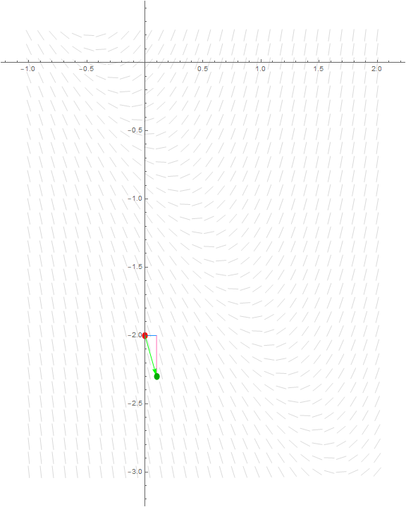
Note that all we did was use the slope of the tangent line through the point \((0, -2)\) to walk a horizontal run of \(0.1\) units, which, directed by the slope of the tangent line, made us drop \(0.3\) units in \(y\). Notice how our walk lies approximately parallel to the line elements around our starting point.

To continue walking through the slope field, we should follow the slope of the tangent line through the new point, since the tangent line through the old point diverges from the true solution. This is how we create a sort of curve: by joining up all of these straight line segments to approximate the true solution. It is not that different from how we manually draw a graph, except that when we manually draw a graph by connecting points, we usually use points that are on the graph of the function. Here, we only have one point that we know for sure is on the actual solution curve: the original point. The rest are only aproximations via tangent lines.

Use our previous ending point as our new starting point, and perform the tangent line approximation again, in order to walk along the tangent line through our new point.

Step Number	Starting Point	Step \[\begin{align*}\color{green}x_{n+1}\color{black} &= \color{red}x_n\color{black} + \color{dodgerblue}\Delta x\color{black}\\\color{green}y_{n+1}\color{black} &= \color{red}y_n\color{black} + f'(\color{red}x_n\color{black})\cdot\color{dodgerblue}\Delta x\color{black}\end{align*}\]	Ending Point
Step 1	\[(x_0, y_0) = (0, -2)\]	\[\begin{align*}\color{green}x_1\color{black} &= \color{red}x_0\color{black} + \color{dodgerblue}\Delta x\color{black}\\&= \color{red}0\color{black} + \color{dodgerblue}0.1\color{black}\\&= \color{green}0.1\color{black}\\\hline\color{green}y_1 \color{black}&= \color{red}y_0\color{black} + f'(\color{red}x_0\color{black})\cdot\color{dodgerblue}\Delta x\color{black}\\&= \color{red}y_0\color{black} + (3\color{red}x_0\color{black} + 2\color{red}y_0\color{black} + 1)\cdot \color{dodgerblue}0.1\color{black}\\&= \color{red}-2\color{black} + (3\cdot \color{red}0\color{black} + 2\cdot \color{red}(-2)\color{black} + 1)\cdot \color{dodgerblue}0.1\color{black}\\&= \color{green}-2.3\color{black}\end{align*}\]	\[(x_1, y_1) = (0.1, -2.3)\]
Step 2	\[(x_1, y_1) = (0.1, -2.3)\]	\[\begin{align*}\color{green}x_2\color{black} &= \color{red}x_1\color{black} + \color{dodgerblue}\Delta x\color{black}\\&= \color{red}0.1\color{black} + \color{dodgerblue}0.1\color{black}\\&= \color{green}0.2\color{black}\\\hline\color{green}y_2 \color{black}&= \color{red}y_1\color{black} + f'(\color{red}x_1\color{black})\cdot\color{dodgerblue}\Delta x\color{black}\\&= \color{red}y_1\color{black} + (3\color{red}x_1\color{black} + 2\color{red}y_1\color{black} + 1)\cdot \color{dodgerblue}0.1\color{black}\\&= \color{red}-2.3\color{black} + (3\cdot \color{red}0.1\color{black} + 2\cdot \color{red}(-2.3)\color{black} + 1)\cdot \color{dodgerblue}0.1\color{black}\\&= \color{green}-2.63\color{black}\end{align*}\]	\[(x_2, y_2) = (0.2, -2.63)\]

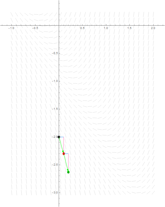
We can see that we are headed pretty much in the same direction as last time. Although this is relatively unexciting, this would bode well for approximation, since there are no nearby graphically obvious changes in the behavior of the derivative, such as the region to the right where we see the graph rapidly changes to curve upwards. Since the derivative does not change much in our region of the graph, our approximation is actually bound to be better than if we had to approximate a value near the curvier portion of the slope field.

We can continue this process indefinitely, to get approximate values of the solution through our original point.

Step Number	Starting Point	Step \[\begin{align*}\color{green}x_{n+1}\color{black} &= \color{red}x_n\color{black} + \color{dodgerblue}\Delta x\color{black}\\\color{green}y_{n+1}\color{black} &= \color{red}y_n\color{black} + f'(\color{red}x_n\color{black})\cdot\color{dodgerblue}\Delta x\color{black}\end{align*}\]	Ending Point
Step 1	\[(x_0, y_0) = (0, -2)\]	\[\begin{align*}\color{green}x_1\color{black} &= \color{red}x_0\color{black} + \color{dodgerblue}\Delta x\color{black}\\&= \color{red}0\color{black} + \color{dodgerblue}0.1\color{black}\\&= \color{green}0.1\color{black}\\\hline\color{green}y_1 \color{black}&= \color{red}y_0\color{black} + f'(\color{red}x_0\color{black})\cdot\color{dodgerblue}\Delta x\color{black}\\&= \color{red}y_0\color{black} + (3\color{red}x_0\color{black} + 2\color{red}y_0\color{black} + 1)\cdot \color{dodgerblue}0.1\color{black}\\&= \color{red}-2\color{black} + (3\cdot \color{red}0\color{black} + 2\cdot \color{red}(-2)\color{black} + 1)\cdot \color{dodgerblue}0.1\color{black}\\&= \color{green}-2.3\color{black}\end{align*}\]	\[(x_1, y_1) = (0.1, -2.3)\]
Step 2	\[(x_1, y_1) = (0.1, -2.3)\]	\[\begin{align*}\color{green}x_2\color{black} &= \color{red}x_1\color{black} + \color{dodgerblue}\Delta x\color{black}\\&= \color{red}0.1\color{black} + \color{dodgerblue}0.1\color{black}\\&= \color{green}0.2\color{black}\\\hline\color{green}y_2 \color{black}&= \color{red}y_1\color{black} + f'(\color{red}x_1\color{black})\cdot\color{dodgerblue}\Delta x\color{black}\\&= \color{red}y_1\color{black} + (3\color{red}x_1\color{black} + 2\color{red}y_1\color{black} + 1)\cdot \color{dodgerblue}0.1\color{black}\\&= \color{red}-2.3\color{black} + (3\cdot \color{red}0.1\color{black} + 2\cdot \color{red}(-2.3)\color{black} + 1)\cdot \color{dodgerblue}0.1\color{black}\\&= \color{green}-2.63\color{black}\end{align*}\]	\[(x_2, y_2) = (0.2, -2.63)\]
Step 3	\[(x_2, y_2) = (0.2, -2.63)\]	\[\begin{align*}\color{green}x_3\color{black} &= \color{red}x_2\color{black} + \color{dodgerblue}\Delta x\color{black}\\ &= \color{green}0.3\color{black}\\\hline\color{green}y_3 \color{black}&= \color{red}y_2\color{black} + f'(\color{red}x_2\color{black})\cdot\color{dodgerblue}\Delta x\color{black}\\ &= \color{green}-2.996\color{black}\end{align*}\]	\[(x_3, y_3) = (0.3, -2.996)\]
Step 4	\[(x_3, y_3) = (0.3, -2.996)\]	\[\begin{align*}\color{green}x_4\color{black} &= \color{red}x_3\color{black} + \color{dodgerblue}\Delta x\color{black}\\ &= \color{green}0.4\color{black}\\\hline\color{green}y_4 \color{black}&= \color{red}y_3\color{black} + f'(\color{red}x_3\color{black})\cdot\color{dodgerblue}\Delta x\color{black}\\ &= \color{green}-3.4052\color{black}\end{align*}\]	\[(x_4, y_4) = (0.4, -3.4052)\]
Step 5	\[(x_4, y_4) = (0.4, -3.4052)\]	\[\begin{align*}\color{green}x_5\color{black} &= \color{red}x_4\color{black} + \color{dodgerblue}\Delta x\color{black}\\ &= \color{green}0.5\color{black}\\\hline\color{green}y_5 \color{black}&= \color{red}y_4\color{black} + f'(\color{red}x_4\color{black})\cdot\color{dodgerblue}\Delta x\color{black}\\ &= \color{green}-3.86624\color{black}\end{align*}\]	\[(x_5, y_5) = (0.5, -3.86624)\]
Step 6	\[(x_5, y_5) = (0.5, -3.86624)\]	\[\begin{align*}\color{green}x_6\color{black} &= \color{red}x_5\color{black} + \color{dodgerblue}\Delta x\color{black}\\ &= \color{green}0.6\color{black}\\\hline\color{green}y_6 \color{black}&= \color{red}y_5\color{black} + f'(\color{red}x_5\color{black})\cdot\color{dodgerblue}\Delta x\color{black}\\ &= \color{green}-4.38949\color{black}\end{align*}\]	\[(x_6, y_6) = (0.6, -4.38949)\]
Step 7	\[(x_6, y_6) = (0.6, -4.38949)\]	\[\begin{align*}\color{green}x_7\color{black} &= \color{red}x_6\color{black} + \color{dodgerblue}\Delta x\color{black}\\ &= \color{green}0.7\color{black}\\\hline\color{green}y_7 \color{black}&= \color{red}y_6\color{black} + f'(\color{red}x_6\color{black})\cdot\color{dodgerblue}\Delta x\color{black}\\ &= \color{green}-4.98739\color{black}\end{align*}\]	\[(x_7, y_7) = (0.7, -4.98739)\]
Step 8	\[(x_7, y_7) = (0.7, -4.98739)\]	\[\begin{align*}\color{green}x_8\color{black} &= \color{red}x_7\color{black} + \color{dodgerblue}\Delta x\color{black}\\ &= \color{green}0.8\color{black}\\\hline\color{green}y_8 \color{black}&= \color{red}y_7\color{black} + f'(\color{red}x_7\color{black})\cdot\color{dodgerblue}\Delta x\color{black}\\ &= \color{green}-5.67487\color{black}\end{align*}\]	\[(x_8, y_8) = (0.8, -5.67487)\]
Step 9	\[(x_8, y_8) = (0.8, -5.67487)\]	\[\begin{align*}\color{green}x_9\color{black} &= \color{red}x_8\color{black} + \color{dodgerblue}\Delta x\color{black}\\ &= \color{green}0.9\color{black}\\\hline\color{green}y_9 \color{black}&= \color{red}y_8\color{black} + f'(\color{red}x_8\color{black})\cdot\color{dodgerblue}\Delta x\color{black}\\ &= \color{green}-6.46984\color{black}\end{align*}\]	\[(x_9, y_9) = (0.9, -6.46984)\]
Step 10	\[(x_9, y_9) = (0.9, -6.46984)\]	\[\begin{align*}\color{green}x_{10}\color{black} &= \color{red}x_9\color{black} + \color{dodgerblue}\Delta x\color{black}\\ &= \color{green}1\color{black}\\\hline\color{green}y_{10} \color{black}&= \color{red}y_9\color{black} + f'(\color{red}x_9\color{black})\cdot\color{dodgerblue}\Delta x\color{black}\\ &= \color{green}-7.39381\color{black}\end{align*}\]	\[(x_{10}, y_{10}) = (1, -7.39381)\]

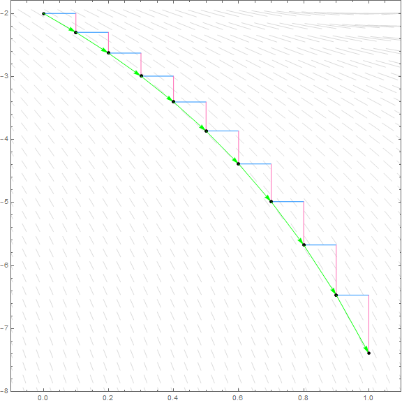
So we have effectively drawn an approximate solution without using any calculus at all: only multiplication and addition. No explicit limits, derivatives, or integrals were necessary. After seeing this, you may wonder why we even bother trying to find an analytic solution to a differential equation, since in many cases the analytic solution is very difficult to visualize or compute specific values for.

Analytic solutions can help us talk about theoretical relationships between solutions when we do not need to find specific values. We can do exact calculus with analytic solutions, for example, but we cannot do it with this approximate graph. So this graphing method is useful for finding approximate specific values when one initial value is known, but is not very good at "the big picture" or talking about more abstract properties of the entire solution (not just a small part of it).

In particular, we should not rely on values after many steps. As we can see from the following graph of the actual solution curve through the point \((0, -2)\), Euler's method diverges significantly from the actual solution curve after many steps, even in relatively calm waters such as these.

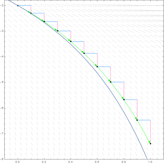
As this differential equation was a first-order linear ordinary differential equation, we were able to find an exact analytic solution using a standard integrating factor.